https://web.stanford.edu/~lutian/coursepdf/

The log-rank Test Assumes More Than the Cox Model – Statistical Thinking

It is well known that the score test for comparing survival distributions between two groups without covariate adjustment, using a Cox proportional hazards (PH) model, is identical to the log-rank \(\chi^2\) test when there are no tied failure times. Yet there persists a belief that the log-rank test is somehow completely nonparametric and does not assume PH. Log-rank and Cox approaches can only disagree if the more commonly used likelihood ratio (LR) statistic from the Cox model disagrees with the log-rank statistic (and the Cox score statistic). This article shows that in fact the log-rank and Cox LR statistics agree to a remarkable degree, and furthermore the hazard ratio arising from the log-rank test also has remarkable agreement with the Cox model counterpart. Since both methods assume PH and the log-rank test assumes within-group heterogeneity (because it doesn’t allow for covariate adjustment), the Cox model actually makes fewer assumptions than log-rank.

https://www.fharrell.com/post/logrank/

t-Test, Chi-Square, ANOVA, Regression, Correlation...

Webapp for statistical data analysis.

https://datatab.net/tutorial/log-rank-test

Log-rank test with a simple example

Let’s start with a simple example. Suppose we have Group 1 and Group 2 and we want to test whether the two groups have the same survival function or not.

In the status, 1 means an event, and 0 means a censored.

There were 6 different time points where events (or censored) were recorded. They are {2, 3, 4, 6, 7, 8}. We do another bookkeeping as following.

Group1 Group2

$m$ counts events and $q$ counts censored. $n$ is for at-risk counts. The interpretation for the first row is as follows: before the time point 2, there were 6 at-risk both in Group 1 and Group 2. There were 1 event in Group 1 and 2 events in Group 2. None was censored in both groups. Likewise, the interpretation of the third row is as follows: there were four individuals at risk in both Group 1 and Group 2. At time point 4, one individual in Group 1 was censored, and two events occurred in Group 2. However, if we refer to the status table above, we see that the censoring actually occurred at time point 5, not 4. Although censored individuals are not counted as events, we include them in the risk set at the immediately preceding time point, rather than at the time they were censored.

If two groups follow the same hazard function, we will estimate that the hazard rate at time 2 is 3/12. It is $(m_1+m_2)/(n_1+n_2).$ So, we calculate the expected number of events by

Note that $m_1+m_2=e_1+e_2$.

We also see that if the hazard rates are same, the difference in $m$ of both groups is just a matter of random split. That is, $m_1$ follows $H(n_1+n_2, m_1+m_2, n_1)$, hypergeometric distribution with the population size of $n_1+n_2$, the success count of $m_1+m_2$, and the draw size of $n_1$.

So the expected value of $m_1$ is

The variance of $m_1$ is

By the Lyapunov central limit theorem,

where

In fact, there is a symmetry in $Var(m_1)$, so $Var(m_1)=Var(m_2)$.

So, $s^2=1.777$ and $s=1.333$.

$z=-1.16/1.333=-0.8702$. So, we won’t be able to reject the null hypothesis.

By the way, $z^2$ follows $\chi^2(1)$.

Let’s see no-roundup calculation using R code.

df <- data.frame(m1=c(1, 1, 0, 0, 2, 1))
df$n1 <- c(6,5,4,3,3,1)
df$m2 <- c(2,0,2,1,0,1)
df$n2 <- c(6,4,4,2,1,1)

df$E <- df$n1*(df$m1 + df$m2)/(df$n1 + df$n2)
df$V <- ( df$n1*df$n2 )/( (df$n1 + df$n2)^2  )*( df$m1 + df$m2 )*(df$n1 + df$n2 -df$m1-df$m2 )/(df$n1 + df$n2 - 1 )

s_square = sum(df$V)
OmE_square = (sum(df$m1 - df$E))^2

z = sqrt(OmE_square/s_square)
chisq_stat = OmE_square/s_square
cat('z =',z)
cat('\nchisq =', chisq_stat)

cat('\np_val_z = ', 2*(1-pnorm(z)))
cat('\np_val_chisq = ', (1-pchisq(chisq_stat, df=1)))

z = 0.8663394
chisq = 0.7505439
p_val_z =  0.3863041
p_val_chisq =  0.3863041

If we use R libraries, we can see familiar numbers.

• R code chunks

  💡

  • Libraries

  library(survival)
  library(survminer)

  💡

  • Create dataset

  #    'time' is the observed time until event or censoring
  #    'event' is the event indicator (1 = event occurred, 0 = censored)
  #    'batch' is a categorical variable for manufacturing batch
  
  simple_data <- data.frame(
    time = c(2, 3, 5, 7, 7, 8,  # Fertilizer X
             2, 2, 4, 4, 6, 8), # Fertilizer Y
    event = c(1, 1, 0, 1, 1, 1,    # Fertilizer X events/censoring
              1, 1, 1, 1, 1, 1),    # Fertilizer Y events/censoring
    group = factor(c(rep("Group 1", 6), rep("Group 2", 6))) # Create factors for groups
  )

  💡

  Create a 'Surv' object

  #    This object combines the time and event status, which is required by
  #    survival analysis functions in R.
  surv_object_simple <- Surv(time = simple_data$time, event = simple_data$event)

  💡

  Kaplan-Meier estimation for overall survival

  km_fit_simple <- survfit(surv_object_simple ~ group, data = simple_data)
  
  # Print the summary of the overall KM fit
  print("Summary of Kaplan-Meier Fit by Group 1 or 2:")
  print(summary(km_fit_simple))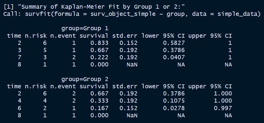

  

  Here, the survival column is the estimated survival function values. The formula is $\hat{S}(t)=\prod (1-m/n)$. The first value of Group 1 is $1-1/6$. The second value is $(1-1/6)(1-1/5)$. The std.err column is calculated by Greenwood’s formula, which is $\hat{\sigma}(t)=\sqrt{ \hat{S}(t)^2\sum m/(n(n-m))}$. The 95% CI calculation has a few options: plain, log, or log-log. It appears that log transformation based method is applied here. The formula is

  $$CI=\exp \Big[\ln\hat{S}(t)\pm z_{1-\alpha/2}\cdot \frac{\hat{\sigma}(t)}{\hat{S}(t)}\Big]$$

  For the first row of Group 1,

  $$CI=\exp \Big[ \ln 0.833 \pm 1.96\cdot0.152/0.833 \Big]=0.58253 \text{ or } 1.19115$$

  sounds about right. For the second row

  $$CI=\exp \Big[ \ln 0.667 \pm 1.96\cdot0.192/0.667 \Big]= 0.3794 \text{ or } 1.17261$$

  also looks correct enough. Which one to use when? Let’s ask chatGPT.

  

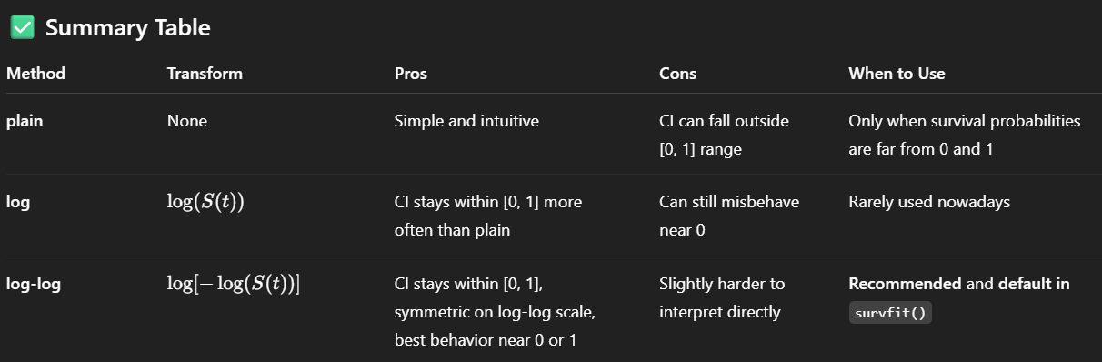
  It sounds like survfit chose something that’s rarely used nowadays.

  💡

  5. Plot the Kaplan-Meier curves by group

  # ggsurvplot from survminer provides a nice, publication-ready plot
  ggsurvplot(km_fit_plant,
  data = plant_data,
  risk.table = TRUE,
  linetype = c(1,4),
  tables.height = 0.3,
  pval = TRUE)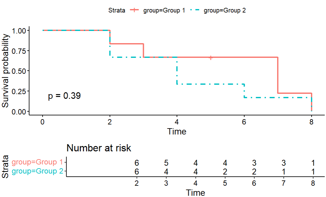

  

More to add with a complex example

• Code chunks

  #https://bookdown.org/drki_musa/dataanalysis/survival-analysis-kaplan-meier-and-cox-proportional-hazard-ph-regression.html#data
  library(here)
  library(tidyverse)
  library(lubridate)
  library(survival)
  library(survminer)
  library(broom)
  library(gtsummary)

  # https://github.com/drkamarul/data-for-RMed/tree/main/data
  stroke <- read_csv(here('.', 'stroke_data.csv'))
  KM <- survfit(Surv(time = time2, event = status == "dead" ) ~ 1, data = stroke)
  summary(KM)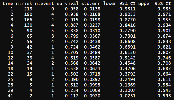

  

  Let try the CI calculation again. The first row:

  $$CI=\exp \Big[ \ln 0.985 \pm 1.96\cdot0.0138/0.985 \Big]=0.93133 \text{ or } 0.98543$$

  looks good.

  # for stoke types
  KM_str_type2 <- survfit(Surv(time = time2, 
                               event = status == "dead" ) ~ stroke_type, 
                          data = stroke)
  summary(KM_str_type2)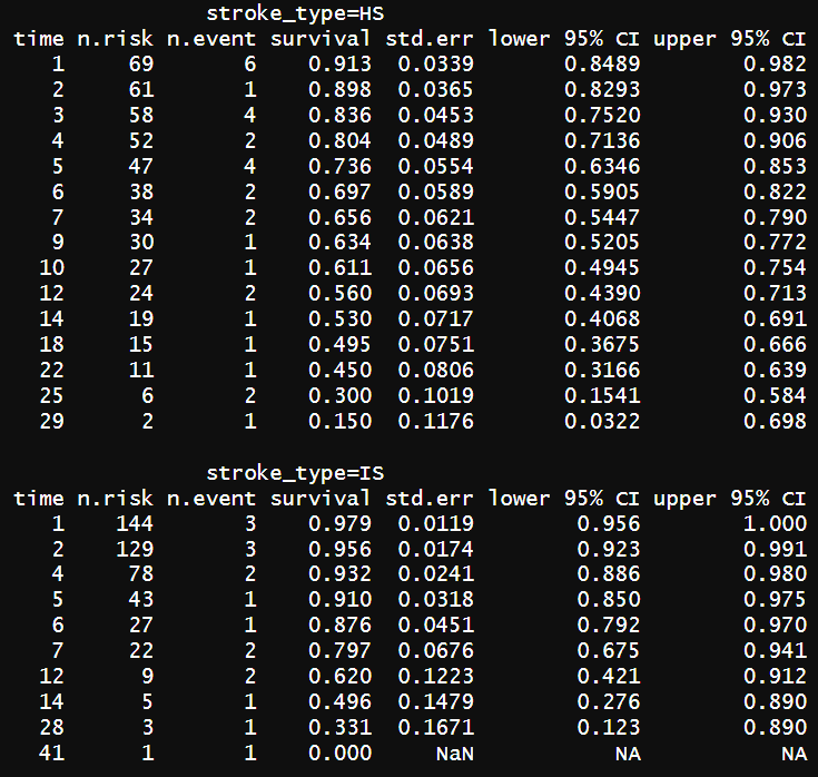

  

  ggsurvplot(KM_str_type2,
             data = stroke,
             risk.table = TRUE,
             linetype = c(1,4),
             tables.height = 0.3,
             pval = TRUE)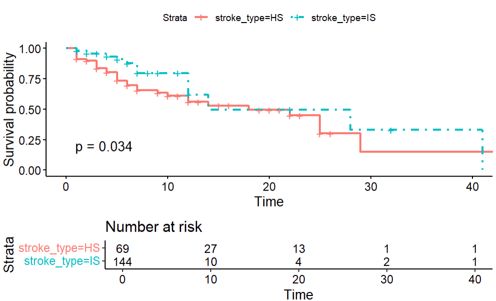

  

  survival functions are different when groups are divided by stroke types.

  #For diebete
  KM_dm <- survfit(Surv(time = time2, 
                        event = status == "dead" ) ~ dm,
                   data = stroke)
  summary(KM_dm)

  ggsurvplot(KM_dm, 
             data = stroke, 
             risk.table = TRUE, 
             linetype = c(1,4), 
             tables.height = 0.3,
             pval = TRUE)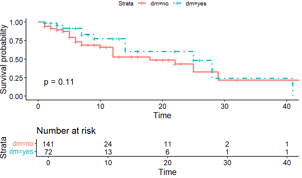

  

  survival functions are not significantly different when groups are divided by dm.

  Log-rank test. (It’s been done already)

  survdiff(Surv(time = time2, 
                event = status == "dead") ~ stroke_type, 
           data = stroke,
           rho = 0)
  ```
  Call:
  survdiff(formula = Surv(time = time2, event = status == "dead") ~ 
      stroke_type, data = stroke, rho = 0)
  
                   N Observed Expected (O-E)^2/E (O-E)^2/V
  stroke_type=HS  69       31     24.2      1.92      4.51
  stroke_type=IS 144       17     23.8      1.95      4.51
  
   Chisq= 4.5  on 1 degrees of freedom, p= 0.03 

  survdiff(Surv(time = time2, 
                event = status == "dead") ~ dm, 
           data = stroke,
           rho = 0)
  ##
  Call:
  survdiff(formula = Surv(time = time2, event = status == "dead") ~ 
      dm, data = stroke, rho = 0)
  
           N Observed Expected (O-E)^2/E (O-E)^2/V
  dm=no  141       35     29.8     0.919      2.54
  dm=yes  72       13     18.2     1.500      2.54
  
   Chisq= 2.5  on 1 degrees of freedom, p= 0.1 

  What is peto-peto test? Let’s see what we get.

  survdiff(Surv(time = time2, 
                event = status == "dead") ~ stroke_type, 
           data = stroke,
           rho = 1)
  ##
  Call:
  survdiff(formula = Surv(time = time2, event = status == "dead") ~ 
      stroke_type, data = stroke, rho = 1)
  
                   N Observed Expected (O-E)^2/E (O-E)^2/V
  stroke_type=HS  69     25.3     18.7      2.33      6.02
  stroke_type=IS 144     13.7     20.3      2.15      6.02
  
   Chisq= 6  on 1 degrees of freedom, p= 0.01 

  Hmm, p-value is lower. Nice!

  survdiff(Surv(time = time2, 
                event = status == "dead") ~ dm, 
           data = stroke,
           rho = 1)
  ##
  Call:
  survdiff(formula = Surv(time = time2, event = status == "dead") ~ 
      dm, data = stroke, rho = 1)
  
           N Observed Expected (O-E)^2/E (O-E)^2/V
  dm=no  141    29.54     24.3      1.11      3.61
  dm=yes  72     9.41     14.6      1.85      3.61
  
   Chisq= 3.6  on 1 degrees of freedom, p= 0.06 

  According to the chatGPT,

  • Peto-Peto (Modified Wilcoxon) Test
    • test for differences between survival curves, but gives more weight to earlier time points
      
      

Dig-ressions

Cox proportional hazards regression

The hazard function is a rate, and because of that it must be strictly positive.

One form of a regression model for the hazard function that addresses the study goal is:

Here, $x$ is variables like certain medical conditions and $\beta$ is a vector of parameters.

• The function, $h_0(t)$, characterizes how the hazard function changes as a function of survival time. baseline hazard function.

• The function, $r(x,\beta)$, characterizes how the hazard function changes as a function of subject covariates, like medical conditions.

The hazard ratio (HR) depends only on the function $r(x,\beta)$.

If the model hazard function is

the hazard ratio is

This model is referred to in the literature by a variety of terms, such as the Cox model, the Cox proportional hazards model or simply the proportional hazards model.

So for example, if we have a covariate which is a dichomotomous (binary), such as stroke type: coded as a value of $x_0=0$ and $x_1=1$, for HS and IS, respectively, then the hazard ratio becomes

If the value of the coefficient is $\beta=\ln(2)$, then the interpretation is that HS are dying at twice ($e^\beta=2$) the rate of patients with IS.

Some disadvantages of KM

• It is a univariable analysis

• It is a non-parametric analysis

We also acknowledge that the fully parametric regression models in survival analysis have stringent assumptions and distribution
requirement. So, to overcome the limitations of the KM analysis and the fully parametric analysis, we can model our survival data using the
semi-parametric Cox proportional hazards regression.

The hazard ratio is 2.75. $h_Y(t)/h_X(t)=2.75$.

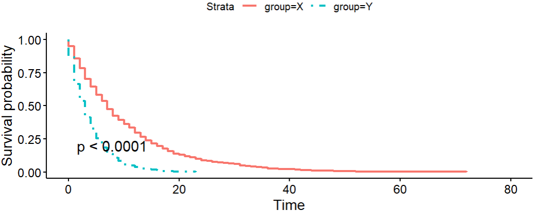
sim_data_coxph <- 
  coxph(Surv(time = time, 
             event = event == 1) ~ group,
                     data = simulated_data)
summary(sim_data_coxph)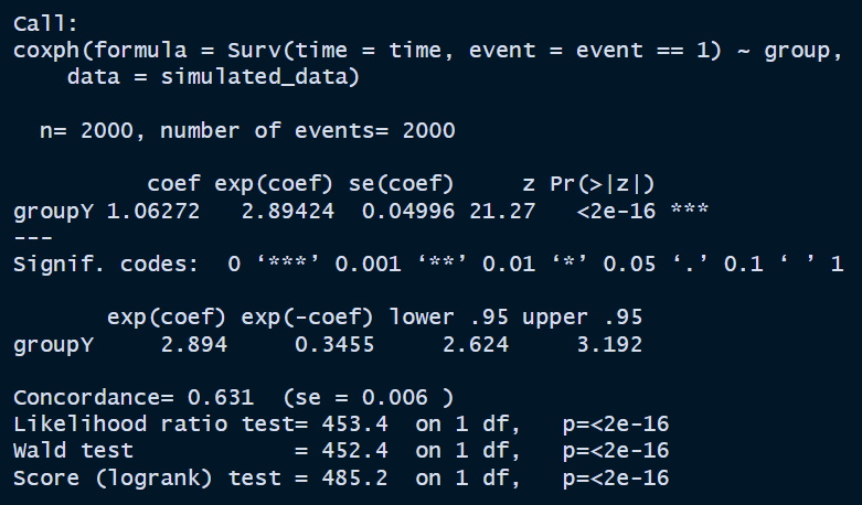

It looks like exp(coef) is very close to 2.75.

Estimation from Cox proportional hazards regression

Simple Cox PH regression

Using our stroke dataset, we will estimate the parameters using the Cox PH regression. Remember, in our data we have

1. the time variable : time2

2. the event variable : status and the event of interest is dead. Event classified other than dead are considered as censored.

3. date variables : date of admission (doa) and date of discharge (dod)

4. all other covariates

stroke_stype <- 
  coxph(Surv(time = time2, 
             event = status == 'dead') ~ stroke_type,
                     data = stroke)
summary(stroke_stype)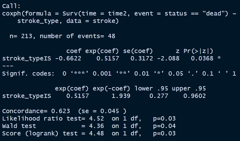

tidy(stroke_stype,
     conf.int = TRUE)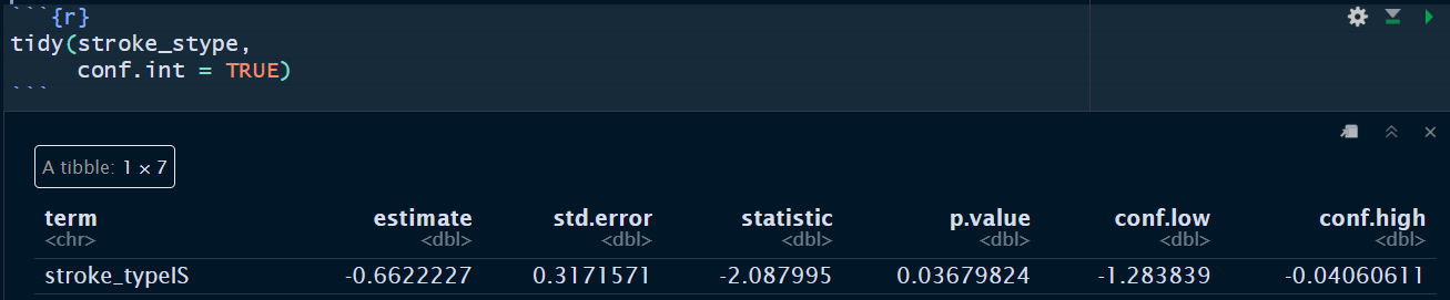

The simple Cox PH model with covariate stroke type shows that the patients with IS has −0.0662 times the crude log hazard for death as compared to patients with HS (p-value = 0.0368).

This means that

and

So, patients with IS survived more.