Digression - simulate survival function

$P(T<t)$: Probability of “death” by time t. $P(T<100)=0.5$ means that half will die by time 100.

$P(T<t)$ is a cumulative distribution of $f(t)=F'(t)$, with $F(t)=P(T<t)$.

$S(t)$: Survival function, $S(t)=1-F(t)=P(T>t)$, probability to survive to time t.

$h(t)$: hazard function. the instantaneous failure rate, scaled by the fraction of surviving systems at time t

This means that

Or,

Let’s simulate a survival data for a simple case.

Let’s suppose that we have a survival data whose hazard function is constant, $h(t)=0.1$.

Since $h(t)=f(t)/S(t)$ and $S(t)$ is a monotone decreasing function, a constant hazard function means that $f(t)$, the probability density function of the even happening, should be also a monotone decreasing function.

By the above formula, $F(t)=1-\exp(-0.1t)$. We will generate event occurring time data by inverse transformation sampling. That means, $F^{-1}(u)$, for u from uniform($[0, 1]$), is a random sample. We will be solving $\exp(-0.1t)=1-u$. By the way, $1-u$ is also a random number from uniform($[0, 1]$). So, we will just solve for $t$ from $\exp(-0.1t)=u$. That is, $t=-\ln(u)/0.1$.

set.seed(5670)
h = 0.1
n <- 20
u <- runif(n)
observed_times <- -log(u)/h
status <- as.numeric(observed_times >-1) # let's assume that non was censored.
surv_obj <- Surv(round(observed_times), status) # observed times are rounded as if the unit of time is one. 
# Fit Kaplan-Meier estimator
fit <- survfit(surv_obj ~ 1)

# Plot survival curve
plot(fit, xlab = "Time", ylab = "Survival Probability", main = "Simulated Survival Curve")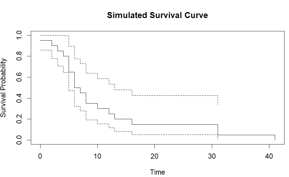

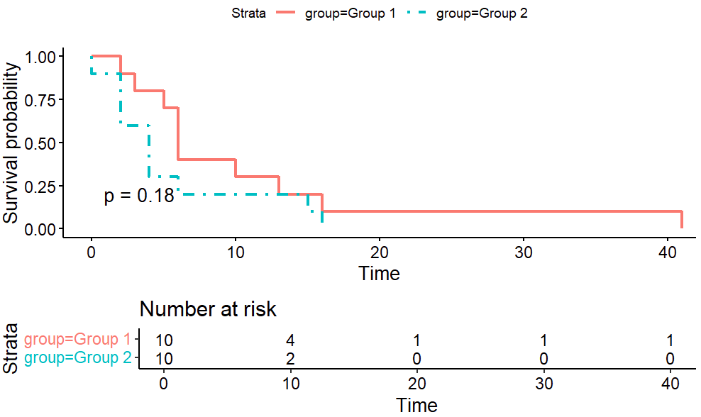
The following is a simulation of two groups one is with $h(t)=0.1$ and the other has $h(t)=0.2$. There are 10 subjects in each group. With a total of 20 subjects, the p-value of log-rank test is 0.18.

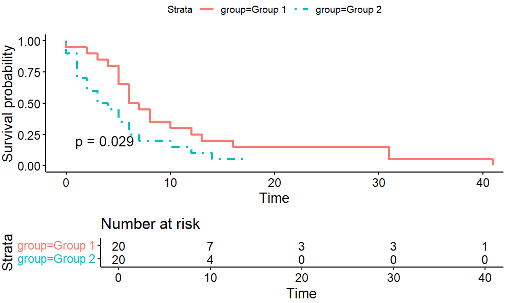
Here we increase the number of subjects to 20 each.

2000 simulated data

Let’s generate 2*1000 simulated data for the Cox proportional hazard regression. Two groups, X and Y have a constant hazard function ratio of 2.75.

# set.seed(5670)
n <- 1000

h = 0.1
u1 <- runif(n)
observed_times1 <- -log(u1)/h


h2 = h*2.75
u2 <- runif(n)
observed_times2 <- -log(u2)/h2


# status <- as.numeric(observed_times >-1)

simulated_data <- data.frame(
  time = round(c(observed_times1, observed_times2)), # Fertilizer Y
  event = rep(1, 2*n),    # Fertilizer Y events/censoring
  group = factor(c(rep("X", n), rep("Y", n))) # Create factors for groups
)

surv_object_simulated <- Surv(time = simulated_data$time, event = simulated_data$event)

# surv_obj <- Surv(round(observed_times), status)
km_fit_simulated <- survfit(surv_object_simulated ~ group, data = simulated_data)

# Print the summary of the overall KM fit

print("Summary of Kaplan-Meier Fit by Group 1 or 2:")
print(summary(km_fit_simulated))