Chi Square Test of Independence
Resources
- https://online.stat.psu.edu/stat500/lesson/8/8.1
- https://en.wikipedia.org/wiki/Chi-squared_test
- https://medium.com/bukalapak-data/meet-the-engine-of-a-b-testing-chi-square-test-30e8a8ab44c5
Pearson’s chi-squared test

Suppose that n observations in a random sample from a population are classified into 2 mutually exclusive classes with respective observed numbers of observations (for ), and a null hypothesis gives the probability that an observation falls into the class. So, we have the expected numbers and .
Let’s suppose that for simplicity and this is the null hypothesis. Pearson proposed that under the null hypothesis and for a large , follows distribution with 1 degree of freedom.
Here is a simulation.
n=1000
nsam=50000
data <- c()

for (ii in 1:nsam){
  samp <- sample(0:1,n, replace=T)
  x1 <- sum(samp)
  x2 <- n - sum(samp)
  chi2 <- (x1 - n/2)**2/(n/2)+(x2 - n/2)**2/(n/2)
  data <- c(data, chi2)
}
hist(data, freq=F, breaks = 67)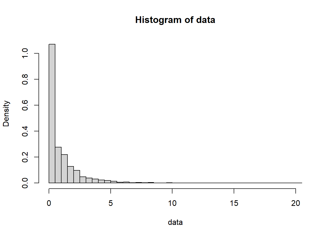
It looks believable. Let’s consider a new problem. Suppose that we sampled 1000 from a population which consists of type A and B, and got 450 type A and 550 type B. Can we say that the proportion of type A and B are not the same in the population?
With the null hypothesis of the same proportion for type A and B, we get the P-value of \[ \frac{(450-500)^2}{500}+\frac{(550-500)^2}{500} = 10 \text{ is}\]
degfree = 1
pval = 1-pchisq(10, df=degfree)
cat(as.character(pval))
0.0015654022580025
It’s pretty low, so we can say that the proportion of type A and B are NOT the same.
We can generalize the earlier statement. The general statement is
8.1 - The Chi-Square Test of Independence
The previous example was about one categorical random variable. This example is about two categorical random variables.
How do we test the independence of two categorical variables? It will be done using the Test of Independence.
As with all prior statistical tests, we need to define null and alternative hypotheses. Also, as we have learned, the null hypothesis is what is assumed to be true until we have evidence to go against it. In this lesson, we are interested in researching if two categorical variables are related or associated (i.e., dependent). Therefore, until we have evidence to suggest that they are, we must assume that they are not. This is the motivation behind the hypothesis for the Chi-Square Test of Independence:
- : In the population, the two categorical variables are independent.
- : In the population, the two categorical variables are dependent.
Note! There are several ways to phrase these hypotheses. Instead of using the words “independent” and “dependent” one could say “there is no relationship between the two categorical variables” versus “there is a relationship between the two categorical variables.” Or “there is no association between the two categorical variables” versus “there is an association between the two variables.” The important part is that the null hypothesis refers to the two categorical variables not being related while the alternative is trying to show that they are related.
Once we have gathered our data, we summarize the data in the two-way contingency table. This table represents the observed counts and is called the Observed Counts Table or simply the Observed Table. The contingency table on the introduction page to this lesson represented the observed counts of the party affiliation and opinion for those surveyed.
The question becomes, “How would this table look if the two variables were not related?” That is, under the null hypothesis that the two variables are independent, what would we expect our data to look like?
Consider the following table:
| Success | Failure | Total | |
| Group1 | | | |
| Group2 | | | |
| Total | | | |
The total count is . Let’s focus on one cell, say Group 1 and Success with observed count . If we go back to our probability lesson, let \(G_1\) denote the event ‘Group 1’ and denote the event ‘Success.’ Then,
Recall that if two events are independent, then their intersection is the product of their respective probabilities. In other words, if and are independent,
So, if and are independent, the expected observation count is
Like this, we can make a table of expected counts:
| Success | Failure | |
|---|---|---|
| Group1 | | |
| Group2 | | |
With observed counts and expected counts under , it is known that
follows with 1 degree of freedom. Let’s run a simulation.
n=1000
nsam=50000
data2 <- c()

for (ii in 1:nsam){
  samp <- sample(0:1, n, replace=T, prob=c(0.2, 0.8))
  g1 = sum(samp)
  g2 = n-sum(samp)
  samp2 <- sample(0:1, g1, replace=T, prob=c(0.4, 0.6))
  o1_s <- sum(samp2)
  o1_f <- g1-sum(samp2)
  samp3 <- sample(0:1, g2, replace=T, prob=c(0.4, 0.6))
  o2_s <- sum(samp3)
  o2_f <- g2-sum(samp3)
  p_s=(o1_s+o2_s)/n
  p_f=(o1_f+o2_f)/n
  p_1=(o1_s+o1_f)/n
  p_2=(o2_s+o2_f)/n
  e1_s=p_1*p_s*n
  e1_f=p_1*p_f*n
  e2_s=p_2*p_s*n
  e2_f=p_2*p_f*n
  X = ((o1_s-e1_s)**2)/e1_s+((o1_f-e1_f)**2)/e1_f +
    ((o2_s-e2_s)**2)/e2_s+((o2_f-e2_f)**2)/e2_f
  data2 <- c(data2, X)
}

hist(data2, freq=F, breaks = 67)
This looks correct.
The statement above can be generalized.
“For two categorical random variables with and categories, if they are independent,
follows distribution with degrees of freedom.”
test statistic
Let’s consider an example.
| Redeem | Not redeem | |
| existing | 1513 | 14133 |
| revamped | 1853 | 13277 |
In the existing website, something was redeemed and not redeemed. The same observation is made in a revamped website. The above table is the result. It looks like the thing is redeemed at a higher rate with the revamped website. Can we say this? We answer this by testing a hypothesis: H0, “The redemption rate is not associated with the website design.” Applying what we learned above, , , , and . And,
So, the statistic is
(1513-1711.218)**2/1711.218+(14133-13934.78)**2/13934.78+(1853-1654.782)**2/1654.782+(13277-13475.2)**2/13475.2[1] 52.43888
The P-value is extremely low. So, our answer to the question is Yes!
degfree = 1
pval = 1-pchisq(52.43888, df=degfree)
cat(as.character(pval) )
4.43867165245138e-13